Metrics

Load Packages

The first step is to load the rTwig package. Real Twig works well when paired with packages from the Tidyverse, so we will also load the dplyr, tidyr, and ggplot packages to help with data manipulation and visualization, ggpubr for multi-panel plots, and rgl for point cloud plotting.

# Load rTwig
library(rTwig)

# Other useful packages
library(rgl)
library(tidyr)
library(dplyr)
library(ggplot2)
library(ggpubr)

Run Real Twig & Calculate Metrics

Next, let’s run Real Twig with run_rtwig() and calculate our tree metrics with tree_metrics().

# File path to QSM
file <- system.file("extdata/QSM.mat", package = "rTwig")

# Correct QSM cylinders
qsm <- run_rtwig(file, twig_radius = 4.23)

# Calculate detailed tree metrics
metrics <- tree_metrics(qsm$cylin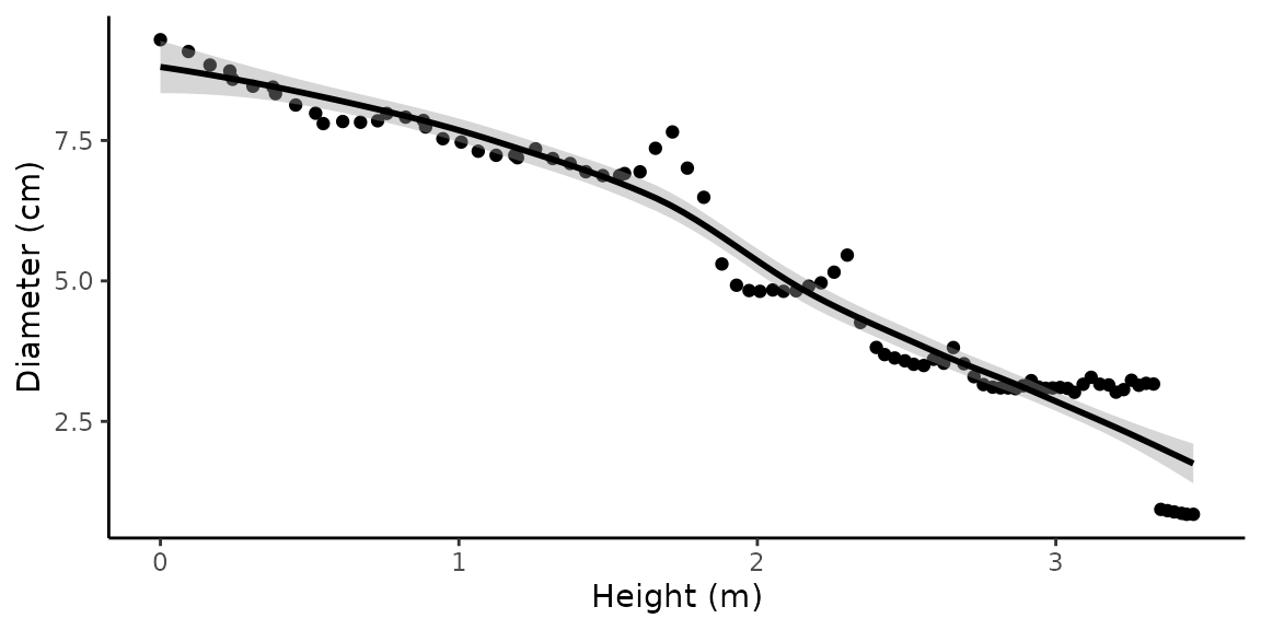der)

Stem Taper

Tree Metrics

Branch Metrics

Segment Metrics

Spreads

Vertical Profile

Point Cloud

We can even plot the simulated point cloud with the rgl library, and look at the cylinder connectivity.

rgl::plot3d(metrics$cloud, aspect = FALSE, decorate = FALSE)
plot_qsm(qsm$cylinder, skeleton = TRUE)

Plotting Code

# Stem Taper -------------------------------------------------------------------
metrics$stem_taper %>%
  ggplot(aes(x = height_m, y = diameter_cm)) +
  geom_point() +
  stat_smooth(method = "loess", color = "black", formula = y ~ x) +
  theme_classic() +
  labs(
    title = "Stem Taper",
    x = "Height (m)",
    y = "Diameter (cm)"
  )

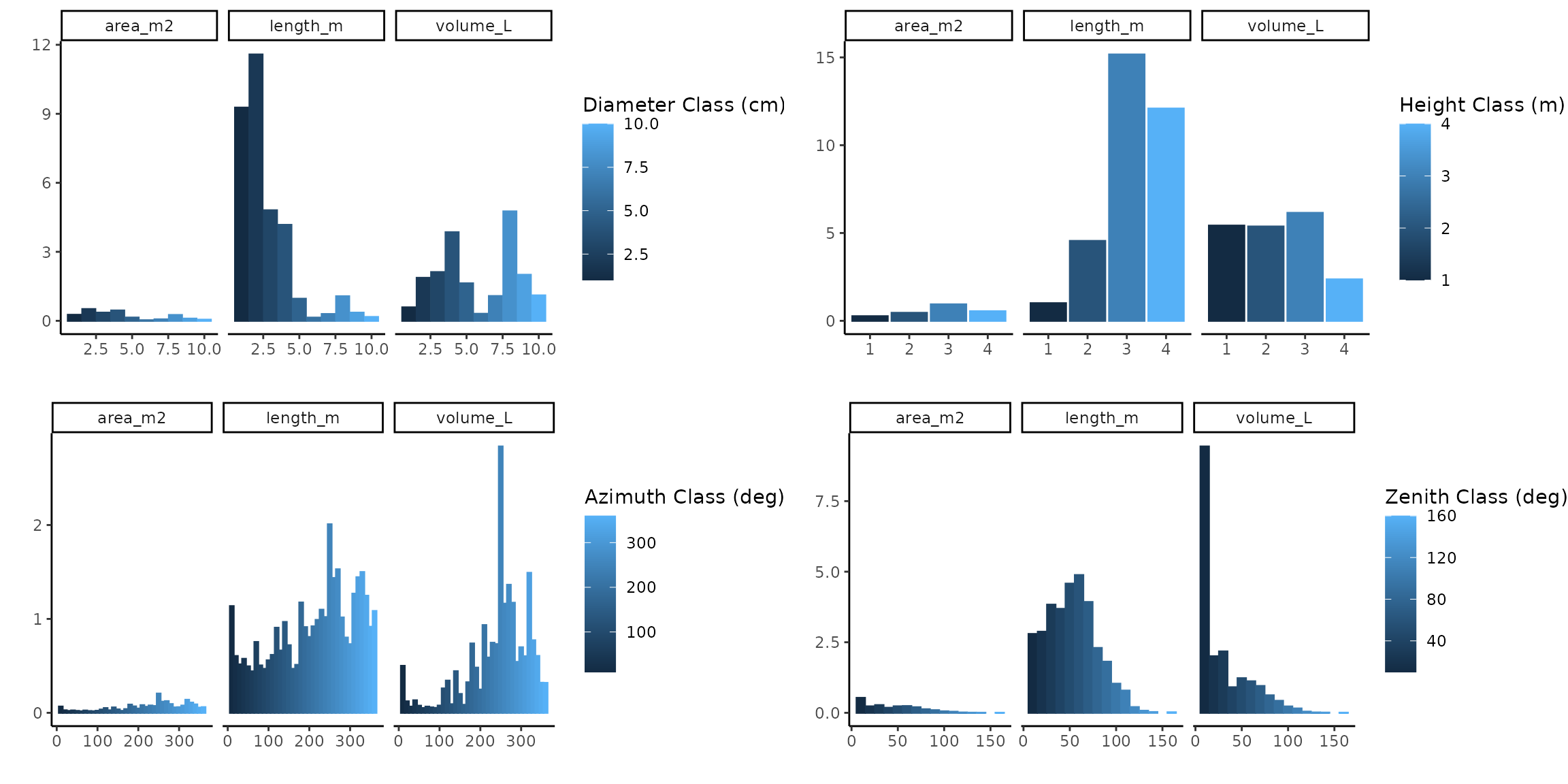
# Tree Metrics -----------------------------------------------------------------
# Tree Height Distributions
metrics$tree_height_dist %>%
  mutate(volume_L = volume_m3 * 1000) %>%
  select(-volume_m3) %>%
  pivot_longer(cols = 2:4, names_to = "type") %>%
  ggplot(aes(
    x = height_class_m,
    y = value,
    color = height_class_m,
    fill = height_class_m
  )) +
  geom_bar(stat = "identity", position = "dodge2") +
  labs(
    title = "Height Distributions",
    x = "",
    y = "",
    fill = "Height Class (m)",
    color = "Height Class (m)"
  ) +
  facet_wrap(~type) +
  theme_classic()

# Tree Diameter Distributions
metrics$tree_diameter_dist %>%
  mutate(volume_L = volume_m3 * 1000) %>%
  select(-volume_m3) %>%
  pivot_longer(cols = 2:4, names_to = "type") %>%
  ggplot(aes(
    x = diameter_class_cm,
    y = value,
    color = diameter_class_cm,
    fill = diameter_class_cm
  )) +
  geom_bar(stat = "identity", position = "dodge2") +
  labs(
     title = "Diameter Distributions",
    x = "",
    y = "",
    fill = "Diameter Class (cm)",
    color = "Diameter Class (cm)"
  ) +
  facet_wrap(~type) +
  theme_classic()

# Tree Zenith Distributions
metrics$tree_zenith_dist %>%
  mutate(volume_L = volume_m3 * 1000) %>%
  select(-volume_m3) %>%
  pivot_longer(cols = 2:4, names_to = "type") %>%
  ggplot(aes(
    x = zenith_class_deg,
    y = value,
    color = zenith_class_deg,
    fill = zenith_class_deg
  )) +
  geom_bar(stat = "identity", position = "dodge2") +
  labs(
    title = "Zenith Distributions",
    x = "",
    y = "",
    fill = "Zenith Class (deg)",
    color = "Zenith Class (deg)"
  ) +
  facet_wrap(~type) +
  theme_classic()

# Tree azimuth distributions
metrics$tree_azimuth_dist %>%
  mutate(volume_L = volume_m3 * 1000) %>%
  select(-volume_m3) %>%
  pivot_longer(cols = 2:4, names_to = "type") %>%
  ggplot(aes(
    x = azimuth_class_deg,
    y = value,
    color = azimuth_class_deg,
    fill = azimuth_class_deg
  )) +
  geom_bar(stat = "identity", position = "dodge2") +
  labs(
    title = "Azimuth Distributions",
    x = "",
    y = "",
    fill = "Azimuth Class (deg)",
    color = "Azimuth Class (deg)"
  ) +
  theme_classic() +
  facet_wrap(~type) +
  theme(legend.position = "right")

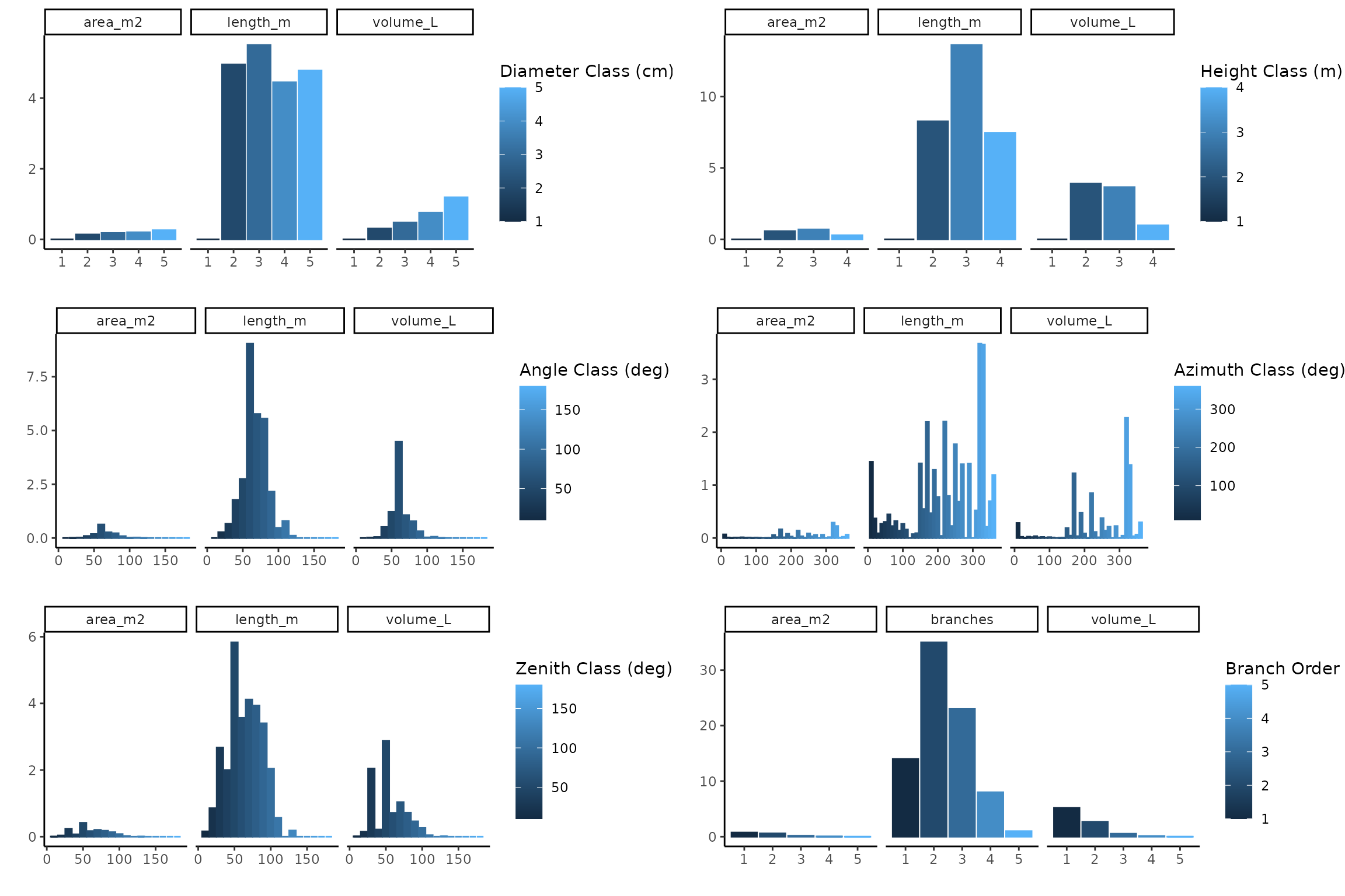
# Branch Metrics ---------------------------------------------------------------
# Branch diameter distributions
metrics$branch_diameter_dist %>%
  mutate(volume_L = volume_m3 * 1000) %>%
  select(-volume_m3) %>%
  relocate(volume_L, .before = area_m2) %>%
  pivot_longer(cols = 2:4, names_to = "type") %>%
  ggplot(aes(
    x = diameter_class_cm,
    y = value,
    color = diameter_class_cm,
    fill = diameter_class_cm
  )) +
  geom_bar(stat = "identity", position = "dodge2") +
  labs(
    title = "Branch Diameter Distributions",
    x = "",
    y = "",
    fill = "Diameter Class (cm)",
    color = "Diameter Class (cm)"
  ) +
  facet_wrap(~type) +
  theme_classic()

# Branch height distributions
metrics$branch_height_dist %>%
  mutate(volume_L = volume_m3 * 1000) %>%
  select(-volume_m3) %>%
  relocate(volume_L, .before = area_m2) %>%
  pivot_longer(cols = 2:4, names_to = "type") %>%
  ggplot(aes(
    x = height_class_m,
    y = value,
    color = height_class_m,
    fill = height_class_m
  )) +
  geom_bar(stat = "identity", position = "dodge2") +
  labs(
    title = "Branch Height Distributions",
    x = "",
    y = "",
    fill = "Height Class (m)",
    color = "Height Class (m)"
  ) +
  facet_wrap(~type) +
  theme_classic()

# Branch angle distributions
metrics$branch_angle_dist %>%
  mutate(volume_L = volume_m3 * 1000) %>%
  select(-volume_m3) %>%
  relocate(volume_L, .before = area_m2) %>%
  pivot_longer(cols = 2:4, names_to = "type") %>%
  ggplot(aes(
    x = angle_class_deg,
    y = value,
    color = angle_class_deg,
    fill = angle_class_deg
  )) +
  geom_bar(stat = "identity", position = "dodge2") +
  labs(
    title = "Branch Angle Distributions",
    x = "",
    y = "",
    fill = "Angle Class (deg)",
    color = "Angle Class (deg)"
  ) +
  facet_wrap(~type) +
  theme_classic()

# Branch zenith distributions
metrics$branch_zenith_dist %>%
  mutate(volume_L = volume_m3 * 1000) %>%
  select(-volume_m3) %>%
  relocate(volume_L, .before = area_m2) %>%
  pivot_longer(cols = 2:4, names_to = "type") %>%
  ggplot(aes(
    x = zenith_class_deg,
    y = value,
    color = zenith_class_deg,
    fill = zenith_class_deg
  )) +
  geom_bar(stat = "identity", position = "dodge2") +
  labs(
    title = "Branch Zenith Distributions",
    x = "",
    y = "",
    fill = "Zenith Class (deg)",
    color = "Zenith Class (deg)"
  ) +
  facet_wrap(~type) +
  theme_classic()

# Branch azimuth distributions
metrics$branch_azimuth_dist %>%
  mutate(volume_L = volume_m3 * 1000) %>%
  select(-volume_m3) %>%
  relocate(volume_L, .before = area_m2) %>%
  pivot_longer(cols = 2:4, names_to = "type") %>%
  ggplot(aes(
    x = azimuth_class_deg,
    y = value,
    color = azimuth_class_deg,
    fill = azimuth_class_deg
  )) +
  geom_bar(stat = "identity", position = "dodge2") +
  labs(
    title = "Branch Azimuth Distributions",
    x = "",
    y = "",
    fill = "Azimuth Class (deg)",
    color = "Azimuth Class (deg)"
  ) +
  facet_wrap(~type) +
  theme_classic()

# Branch order distributions
metrics$branch_order_dist %>%
  mutate(volume_L = volume_m3 * 1000) %>%
  select(-volume_m3) %>%
  relocate(volume_L, .before = area_m2) %>%
  pivot_longer(cols = 2:4, names_to = "type") %>%
  ggplot(aes(
    x = branch_order,
    y = value,
    color = branch_order,
    fill = branch_order
  )) +
  geom_bar(stat = "identity", position = "dodge2") +
  labs(
    title = "Branch Order Distributions",
    x = "",
    y = "",
    fill = "Branch Order",
    color = "Branch Order"
  ) +
  facet_wrap(~type) +

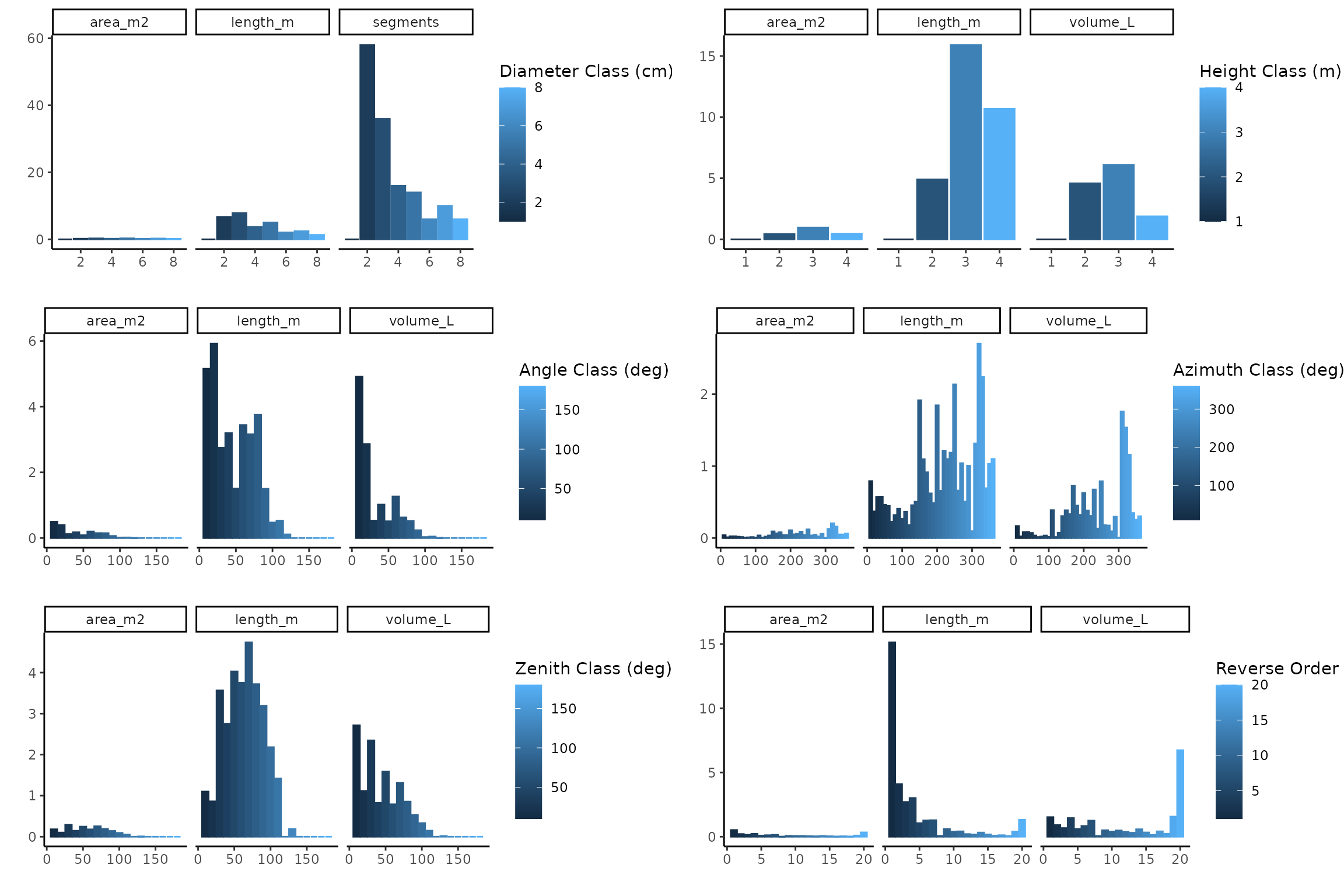
# Segment Metrics --------------------------------------------------------------
# Segment diameter distributions
metrics$segment_diameter_dist %>%
  mutate(volume_L = volume_m3 * 1000) %>%
  select(-volume_m3) %>%
  relocate(volume_L, .before = area_m2) %>%
  pivot_longer(cols = 3:5, names_to = "type") %>%
  ggplot(aes(
    x = diameter_class_cm,
    y = value,
    color = diameter_class_cm,
    fill = diameter_class_cm
  )) +
  geom_bar(stat = "identity", position = "dodge2") +
  labs(
    title = "Segment Diameter Distributions",
    x = "",
    y = "",
    fill = "Diameter Class (cm)",
    color = "Diameter Class (cm)"
  ) +
  facet_wrap(~type) +
  theme_classic()

# Segment height distributions
metrics$segment_height_dist %>%
  mutate(volume_L = volume_m3 * 1000) %>%
  select(-volume_m3) %>%
  relocate(volume_L, .before = area_m2) %>%
  pivot_longer(cols = 2:4, names_to = "type") %>%
  ggplot(aes(
    x = height_class_m,
    y = value,
    color = height_class_m,
    fill = height_class_m
  )) +
  geom_bar(stat = "identity", position = "dodge2") +
  labs(
    title = "Segment Height Distributions",
    x = "",
    y = "",
    fill = "Height Class (m)",
    color = "Height Class (m)"
  ) +
  facet_wrap(~type) +
  theme_classic()

# Segment angle distributions
metrics$segment_angle_dist %>%
  mutate(volume_L = volume_m3 * 1000) %>%
  select(-volume_m3) %>%
  relocate(volume_L, .before = area_m2) %>%
  pivot_longer(cols = 2:4, names_to = "type") %>%
  ggplot(aes(
    x = angle_class_deg,
    y = value,
    color = angle_class_deg,
    fill = angle_class_deg
  )) +
  geom_bar(stat = "identity", position = "dodge2") +
  labs(
    title = "Segment Angle Distributions",
    x = "",
    y = "",
    fill = "Angle Class (deg)",
    color = "Angle Class (deg)"
  ) +
  facet_wrap(~type) +

# Segment zenith distributions
metrics$segment_zenith_dist %>%
  mutate(volume_L = volume_m3 * 1000) %>%
  select(-volume_m3) %>%
  relocate(volume_L, .before = area_m2) %>%
  pivot_longer(cols = 2:4, names_to = "type") %>%
  ggplot(aes(
    x = zenith_class_deg,
    y = value,
    color = zenith_class_deg,
    fill = zenith_class_deg
  )) +
  geom_bar(stat = "identity", position = "dodge2") +
  labs(
    title = "Segment Zenith Distributions",
    x = "",
    y = "",
    fill = "Zenith Class (deg)",
    color = "Zenith Class (deg)"
  ) +
  facet_wrap(~type) +
  theme_classic()

# Segment azimuth distributions
metrics$segment_azimuth_dist %>%
  mutate(volume_L = volume_m3 * 1000) %>%
  select(-volume_m3) %>%
  relocate(volume_L, .before = area_m2) %>%
  pivot_longer(cols = 2:4, names_to = "type") %>%
  ggplot(aes(
    x = azimuth_class_deg,
    y = value,
    color = azimuth_class_deg,
    fill = azimuth_class_deg
  )) +
  geom_bar(stat = "identity", position = "dodge2") +
  labs(
    title = "Segment Azimuth Distributions",
    x = "",
    y = "",
    fill = "Azimuth Class (deg)",
    color = "Azimuth Class (deg)"
  ) +
  facet_wrap(~type) +
  theme_classic()

# Segment order distributions
metrics$segment_order_dist %>%
  mutate(volume_L = volume_m3 * 1000) %>%
  select(-volume_m3) %>%
  relocate(volume_L, .before = area_m2) %>%
  pivot_longer(cols = 3:5, names_to = "type") %>%
  ggplot(aes(
    x = reverse_order,
    y = value,
    color = reverse_order,
    fill = reverse_order
  )) +
  geom_bar(stat = "identity", position = "dodge2") +
  labs(
    title = "Reverse Order Distributions",
    x = "",
    y = "",
    fill = "Reverse Order",
    color = "Reverse Order"
  ) +
  facet_wrap(~type) +
  theme_classic()

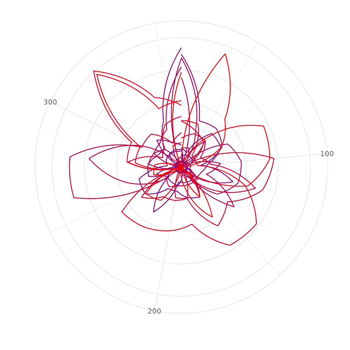
# Spreads ----------------------------------------------------------------------
spreads <- metrics$spreads

# Generate colors from red to blue
n <- length(unique(spreads$height_class))
colors <- data.frame(r = seq(0, 1, length.out = n), g = 0, b = seq(1, 0, length.out = n))

# Convert colors to hex
color_hex <- apply(colors, 1, function(row) {
  rgb(row[1], row[2], row[3])
})

# Assign colors to height classes
height_class_colors <- data.frame(
  height_class = unique(spreads$height_class),
  color = color_hex
)

spreads %>%
  left_join(height_class_colors, by = "height_class") %>%
  ggplot(aes(x = azimuth_deg, y = spread_m, group = height_class, color = color)) +
  geom_line() +
  scale_color_identity() +
  coord_polar(start = 0) +
  labs(x = "", y = "") +
  theme_minimal() +
  theme(axis.text.y = element_blank())

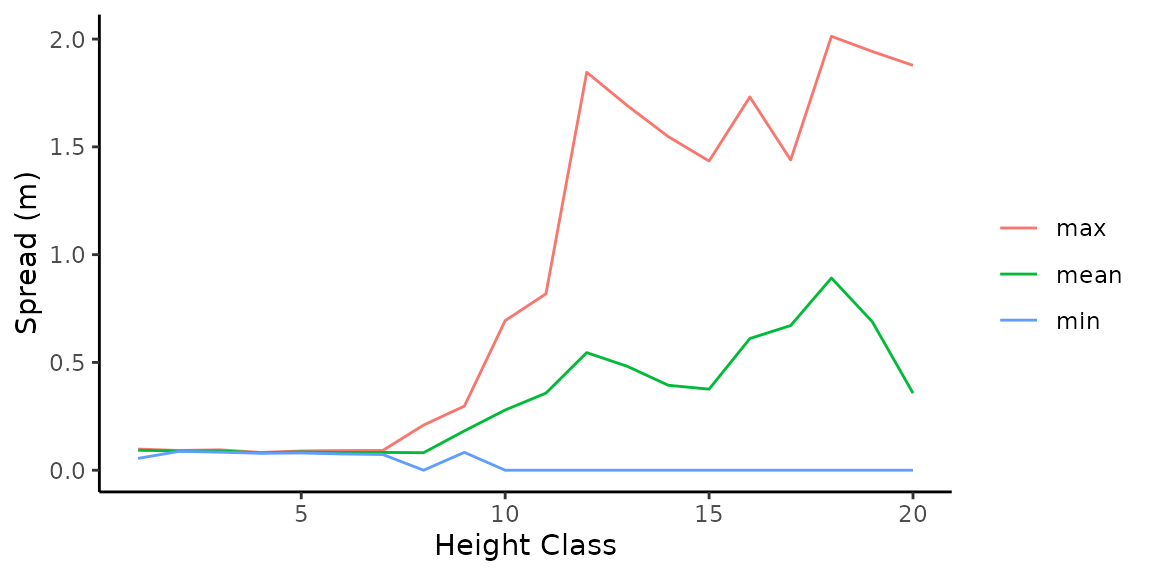
# Vertical profile -------------------------------------------------------------
metrics$spreads %>%
  group_by(height_class) %>%
  summarize(
    max = max(spread_m),
    mean = mean(spread_m),
    min = min(spread_m)
  ) %>%
  pivot_longer(cols = 2:4, names_to = "type") %>%
  ggplot(aes(x = height_class, y = value, color = type)) +
  geom_line() +
  labs(
    x = "Height Class",
    y = "Spread (m)",
    color = ""
  ) +
  theme_classic()